Linear regression, a widely used supervised machine learning technique, harnesses labeled datasets to forecast future outcomes and uncover valuable insights. Renowned for its predictive prowess, this algorithm empowers businesses to anticipate sales trends, preempt potential losses, and make informed decisions.

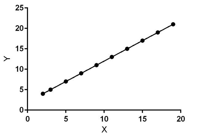
Imagine a graph displaying training data points plotted against specific values. These data points serve as the foundation for predicting future trends and outcomes, enabling businesses to make informed decisions.

Let us delve into the formula used for calculating linear regression:

F(x) = w * x + b

Within this equation, the parameters w and b hold significance, representing the coefficients, while x symbolizes the feature being evaluated.

Let’s explore how this formula is implemented in programming to bring these concepts to life.

w=1.0
b=2.0
x = np.array([1, 2, 3, 4, 5])
f_x=0
for i in range(len(x)):
  f_x=w*x[i]+b

Now that we’ve derived the predicted values through f(x), it’s crucial to delve into the concept of the cost function, a pivotal element in the realm of linear regression.

Unveiling the Essence of Cost Function: A Vital Component in the Machinery of Linear Regression

The cost function is an indispensable component of machine learning, serving as a compass to evaluate the performance of our model and guiding us towards improvement by minimizing errors.

Here's a breakdown of the cost function formula: The summation symbol (∑) signifies that we're evaluating the error for each individual data point in our training set.

• y(i) represents the actual values from our training set.

• y^(i) represents the predicted values, typically obtained as the output of our predictive model f(x).

• m denotes the total number of training data points.

Now, let’s delve into how this concept translates into code.

w=1.0
b=2.0
x = np.array([1, 2, 3, 4, 5])
f_x=0
m=len(x)
cost=0
total_cost=0
for i in range(m):
  f_x=w*x[i]+b
   cost = (1/(2*m)) * (x[i] - f_x)**2
   total_cost += cost

Unraveling Gradient Descent: Navigating the Optimization Landscape in Linear Regression

Sure, here’s a simplified version suitable for your blog:

“In linear regression, gradient descent is a vital optimization technique for refining our model’s performance. It works by iteratively adjusting the parameters (weights and biases) to minimize the cost function, which measures the disparity between predicted and actual values.

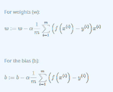
The update formulas for the parameters are:

• w represents the weights,

• b represents the bias,

• α is the learning rate (a small positive value),

• m is the number of training examples,

• f(x(i)) is the predicted value for the ii-th example,

• y(i) is the actual target value for the ii-th example, and

• x(i) is the feature vector for the ii-th example.

This formula directly incorporates the difference between the predicted and actual values (the cost) in the update process for the parameters, aiming to minimize the overall cost function during training.

Let’s demystify this process with code:

w=1.0
b=2.0
x = np.array([1, 2, 3, 4, 5])
f_x=0
dw = 0
db = 0
m=len(x)
cost=0
total_cost=0
for i in range(m):
   f_x=w*x[i]+b
   cost = (1/(2*m)) * (x[i] - f_x)**2
   total_cost += cost
   dw += -(1/len(x)) * x[i] * (y[i] - f_x)
    db += -(1/len(x)) * (y[i] - f_x)